

Programming Language: Python [Link App]
1. Introduction
2. Problem statement
3. The solution
3.1. Building an application + Features
4. Future work ideas
5. Code source
Mining Engineers, and this is my kindly opinion, have learned about solving the Ultimate Pit Limit Problems by easy examples, i.e., Lerchs-Grossman 2D Algorithm. However, that is not what we see when running an open-pit mining operation. Software programs have solved most of the current problems, including this, and some mining engineers become users rather than doers. That being said, I decided to code the solution to the ultimate pit limit problem by applying the Pseudoflow algorithm (Hochbaum, 2008 [0]).
Given a 3D block model, how do we find the economic envelope/volume that contains the maximum value and fits within our operational constraints? i.e., maximum slope angles?
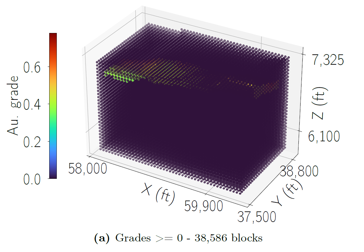 |  | |
|---|---|---|
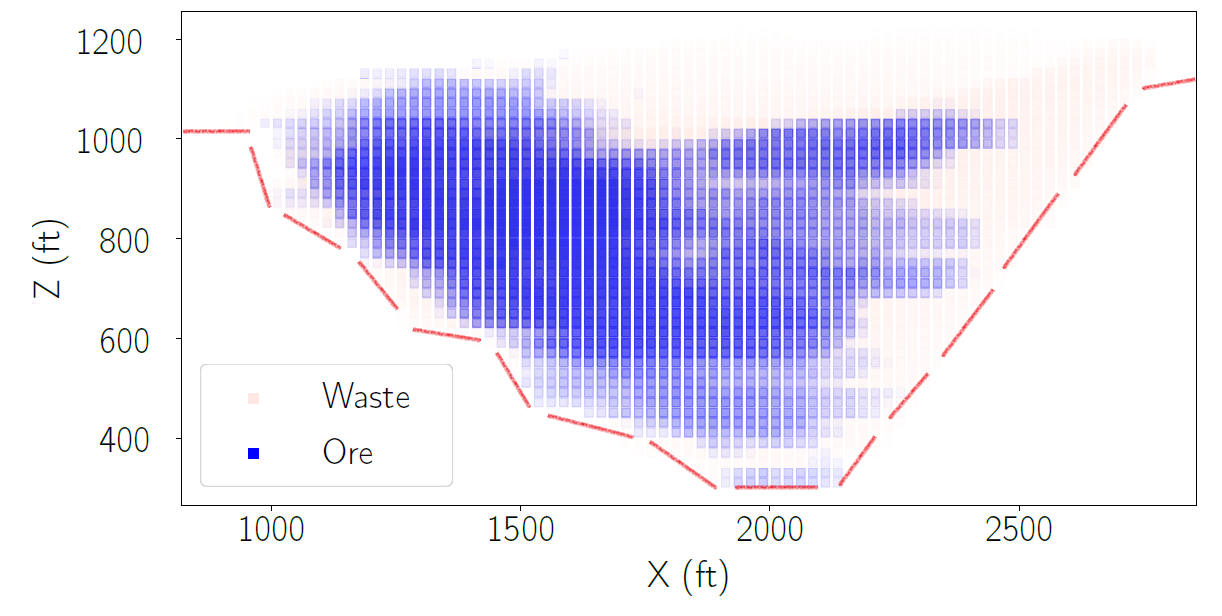
| 3D Block Model | Ultimate Pit Limit |
The solution follows a paper from Geovia Whittle, published in 2017. They explain how the Pseudoflow algorithm works in detail (Geovia, 2017 [1]). To make life easier, this is a summary on how the algorithm works:
1- Estimate each block’s value based on economic parameters:
Cutoff Grade = (MiningCost + ProcessingCost*(1 + Dilution))/(MetalPrice*Recovery)
for block in [1 ... Blocks]:
  block_value = (grade_of_block*Recovery*MetalPrice - (ProcessingCost+MiningCost))*Tons
  if grade_of_block < CutoffGrade:
    block_value = -MiningCost*Tons
2- Create a directed graph with our block model. For that:
if the block's value is positive; the edge’s weight will be the block value.if allowed by the precedence, i.e, 1-5 precedence (45 degrees); the edge’s weight will be the block value.if the block's value is negative; the edge’s weight will be the block value (negative).Hint: You can use ‘Networkx’ to build your graph or do it by your own using dictionaries in Python.
def create_graph(self, bmodel, precedence):
    # Create an empty directed graph.
    Graph = NetX.DiGraph()
    if precedence == 9:
        distance = (self.modex**2 + self.modey**2+ self.modez**2)**0.5
    elif precedence == 5:
        distance = (self.modex**2 + self.modez**2)**0.5
    for step in range(steps_z):
        upper_bench = np.array(bmodel[bmodel.iloc[:,3]== col_compare[step]])
        lower_bench = np.array(bmodel[bmodel.iloc[:,3] == col_compare[step]])
        self.create_edges(
          Graph=Graph, up=upper, low =lower, trigger=step, prec=precedence, dist=distance)
        # Shrink the block model when going down - it reduces the computational time.
        bmodel = bmodel[
          (bmodel.iloc[:,1]!= self.minx+i*self.modex)
          &(bmodel.iloc[:,1]!=self.maxx-i*self.modex)
          &(bmodel.iloc[:,2] != self.miny+i*self.modey)
          &(bmodel.iloc[:,2] != self.maxy-i*self.modey)]
    return Graph

def create_edges(self,Graph,up, low, trigger, prec, dist):
    # Create internal edges - Block to block.
    tree_upper = spatial.cKDTree(up[:,1:4])
    # Get the closest block for each block, yet complying the precedences.
    mask = tree_upper.query_ball_point(low[:,1:4], r = dist + 0.01)
    for _, g in enumerate(mask):
        if len(g) == prec:
            for reach in up[g][:,0]:
              # Add internal edge + adding a weight of 99e9 (infinite).
                Graph.add_edge(low[_][0], reach, const = 99e9, mult = 1)
    #Create external edges - Source to block to sink.
    player = up
    for node, capacity in zip(player[:,0], player[:,4]):
        cap_abs = np.absolute(np.around(capacity, decimals=2))
        # Create an edge from a node to the sink if bvalue less than 0
        if capacity < 0:
            Graph.add_edge(node, self.sink, const = cap_abs, mult = -1)
        # Otherwise the source is connected to the block.
        else:
            Graph.add_edge(0, node, const = cap_abs, mult = 1)
3- The algorithm will push the flow from the source to an ore node and it will try to saturate the capacity. Furthermore, it will push from the waste node to pay for waste blocks. Therefore, as the maximum flow is found, the problem is solved and that will mean that waste blocks were paid. The following chart extracted from ‘Whittle’s paper’ would help you better understand what is written above:
 |
|---|
| Flow going through the graph |
To solve this problem dynamically, and also to make people playing with it, a web application has been created by using Streamlit.
Features of the Application:
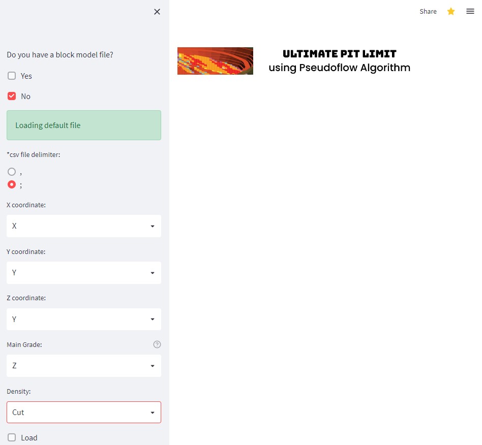 |
|---|
| Uploading a block model file |
It can check outliers after you upload a block model in .csv format. If you do not have it, use a default one. We have everything for you!
3D Visualization: Select some lower and upper bounds for what you want to see and grades’ ranges and we will color-code based on it.
 |
|---|
| 3D Block Model Visualization |
 |
|---|
| Grade-Tonnage Distribution |
 |
|---|
| User Inputs - Economic Parameters |
 |
|---|
| User Inputs - Economic Parameters |